by Thomas Arend

Abstract

The Keeling Curve is a well-known time series that depicts the monthly measurements of atmospheric carbon dioxide (CO₂ ) concentration at the Mauna Loa Observatory (MLO) in Hawaii. This study aims to develop an approximation model for the monthly data of the Keeling Curve by combining exponential and sinusoidal functions to capture both the long-term trend and the annual and semiannual oscillations (SAO).

By fitting the proposed model to the monthly data, the mean difference between the Keeling Curve and the approximation is found to be nearly 0 ppm (-1.462855e-15), indicating a close agreement between the two. Moreover, the standard deviation of the difference is calculated to be 0.7314717 ppm, highlighting the accuracy of the approximation in capturing the variability of the Keeling Curve data.

The developed approximation model provides valuable insights into the behavior of atmospheric CO₂ concentration, allowing for the identification of underlying patterns and trends. It serves as a useful tool for understanding the impact of human activities and natural processes on CO₂ levels in the atmosphere.

Overall, the proposed model successfully approximates the monthly data of the Keeling Curve, providing a comprehensive representation of the long-term trend and the annual and semiannual oscillations in atmospheric CO₂ concentration.

Introduction

The Keeling Curve, initiated by Dr. Charles David Keeling in 1958¹, is a seminal dataset that has provided valuable insights into the increase of atmospheric CO₂ concentration over the past six decades. The curve exhibits a clear upward trend, mainly driven by human activities, superimposed with seasonal variations due to natural processes such as plant growth and decay.

In this study we develop an approximation of the Keeling Curve. For our investigation, we’ll use the monthlyin-situ CO₂ data set that has the file name of »monthly_in_situ_co2_mlo.csv.« We downloaded this file from https://scrippsco2.ucsd.edu/data/atmospheric_co2/primary_mlo_co2_record.html

Antonio Stark² modeled the Keeling Curve with Quadratic Base and Sinusoidal Seasonal Trends. Instead of the quadratic base we will use a exponential base.

Ern et al. (2021)³ investigated the SAO in four different reanalyses for the period 2002–2018 but did not look at CO₂ concentrations.

Jiang et al. (2011)⁴ investigated the CO₂ SOA in the middle troposphere and at the surface. Using in situ measurements, they found a SAO in the midtropospheric and surface CO₂.

Buermann et al (2007)⁵ found that after increasing trends in the seasonal amplitude of CO₂ at the MLO from the early 1970s to the early 1990s an updated record from the MLO indicates that the amplitude of the CO₂ seasonal cycle has been declining since the early 1990s until 2005. For our approximation we will ignore these trends.

1C. D. Keeling, S. C. Piper, R. B. Bacastow, M. Wahlen, T. P. Whorf, M. Heimann, and H. A. Meijer, Exchanges of atmospheric CO₂ and CO₂ with the terrestrial biosphere and oceans from 1978 to 2000. I. Global aspects, SIO Reference Series, No. 01-06, Scripps Institution of Oceanography, San Diego, 88 pages, 2001.

2Antonio Stark: Using Data Science to Understand Climate Change: Atmospheric CO2 Levels (Keeling Curve) — Model Fitting and Time Series Analysis — Published in Towards Data Science, Jun 10, 2020

3Ern, M., Diallo, M., Preusse, P., Mlynczak, M. G., Schwartz, M. J., Wu, Q., and Riese, M.: The semiannual oscillation (SAO) in the tropical middle atmosphere and its gravity wave driving in reanalyses and satellite observations, Atmos. Chem. Phys., 21, 13763–13795, https://doi.org/10.5194/acp-21-13763-2021, 2021.

4Jiang, X., M. T. Chahine, Q. Li, M. Liang, E. T. Olsen, L. L. Chen, J. Wang, and Y. L. Yung (2012), CO2 semiannual oscillation in the middle troposphere and at the surface, Global Biogeochem. Cycles, 26, GB3006, doi:10.1029/2011GB004118.

5Wolfgang Buermann, Benjamin R. Lintner, Charles D. Koven, Alon Angert, Jorge E. Pinzon, Compton J. Tucker, and Inez Y. Fung, The changing carbon cycle at Mauna Loa Observatory, March 13, 2007 104 (11) 4249-4254 doi.org/10.1073/pnas.0611224104.

Methods

To approximate the monthly data (until 04/2023) of the Keeling Curve, we propose a mathematical model that combines an exponential function to capture the long-term trend and sinusoidal functions to represent the seasonal variations. The exponential function reflects the increasing CO2 concentration over time, while the first sinusoidal function accounts for the annual oscillations. The second sinusoidal function accounts for the semiannual oscillations, which were discovered during the modeling process. We will come to this later.

The general form of our model is given by:

CO_{2 (2023)}(t) = A * exp(r * t) + B₁ * sin(2π * (t + φ₁) )+ B₂ * sin(4π * (t + φ₂) )+ C + ε₃(t)

where:

• (t) represents the estimated CO₂ concentration at time t (in decimal date),
• A represents the base level of CO₂ concentration,
• r is the exponential growth rate,
• B1 represents the amplitude of the first sinusoidal function
• B2 represents the amplitude of the second sinusoidal function
• φ1 represents the phase shift of the first sinusoidal function,
• φ2 represents the phase shift of the second sinusoidal function,
• C = C₁ + C₂ + C₃ represents the baseline offset, and
• ε_i(t) represents the remaining error.

To determine the model parameters (A, r, B₁, B₂ , φ₁, φ₂ and C), we employ a curve fitting technique, such as nonlinear least squares regression, to fit the model to the monthly data of the Keeling Curve. We will call this model Model 2023 because we used data from 1958 until April 2023.

In a first step we determine the model parameters for the exponential part of function.

CO₂(t) = A * exp(r * t) +C₁ + ε₁(t)

After building the difference between the values and the exponential approximation ε₁(t) we determine the model parameters for the first sinusoidal function.

ε₁(t)= B₁ * sin(2π * (t + φ₁) )+ C₂ + ε₂(t)

Calculating the error and studying ε₂(t) we found that the error can be further approximated with semiannual sinusoidal function.

Finally we approximate ε₂(t) = B₂ * sin(2π * (t + φ₂)) + C₃ + ε₃(t).

Results

By fitting the proposed model to the monthly data of the Keeling Curve, we obtain estimates for the model parameters. The exponential component captures the long-term trend, while the sinusoidal component captures the seasonal variations. The goodness-of-fit of the model is assessed using statistical measures such as the coefficient of determination (R²) and root mean square error (RMSE).

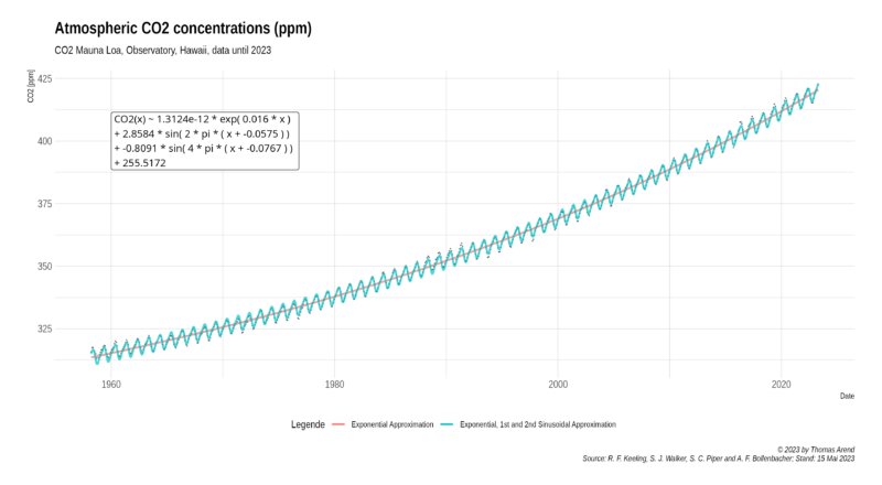
CO2(t) = 1.31242863505765e-12 * exp( 0.0160453592326617 * t )
+ 2.85842937143706 * sin( 2 * pi * ( t - 0.0575 ) )
- 0.809084912332627 * sin( 2 * pi * ( t - 0.0767 ) )
+ 255.517201337755 +ε3( t )

We found R² = 0.9934622 for the exponential part, R² = 0.8256447 for the first and R² = 0.3814435 for the second sinusoidal part of the approximation function.

The mean difference between the Keeling Curve and the exponential approximation (ε₁(t)) is found to be 0.03429826. The standard deviation of the difference is calculated to be 2.22735962.

Adding 1^st sinusoidal part for the annual variations reduces the mean of the difference to nearly 0 (1.646100e-14) and the standard deviation is reduced to 0.9300533.

When adding the 2^nd sinusoidal part for the semi-annual variations the mean difference (ε₃(t)) is found to be nearly 0 (-1.624126e-14), indicating a close agreement between the two. Moreover, the standard deviation of the difference is reduced to 0.7314717 indicating that the approximation effectively captures the variability in the Keeling Curve data.

Four diagrams will be included to illustrate the results:

Keeling Curve

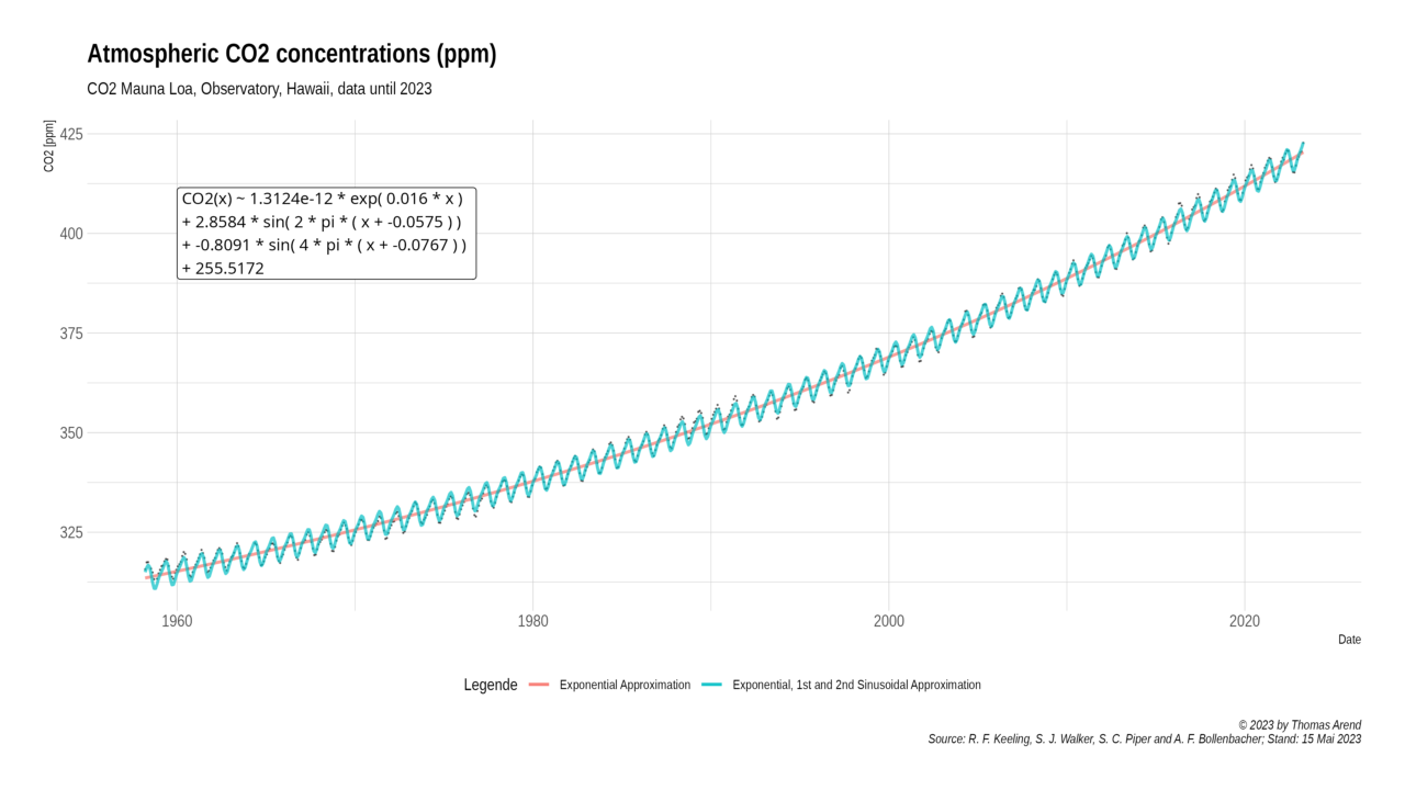
Diagram 1: Keeling Curve with Approximations

Error ε₁(t)

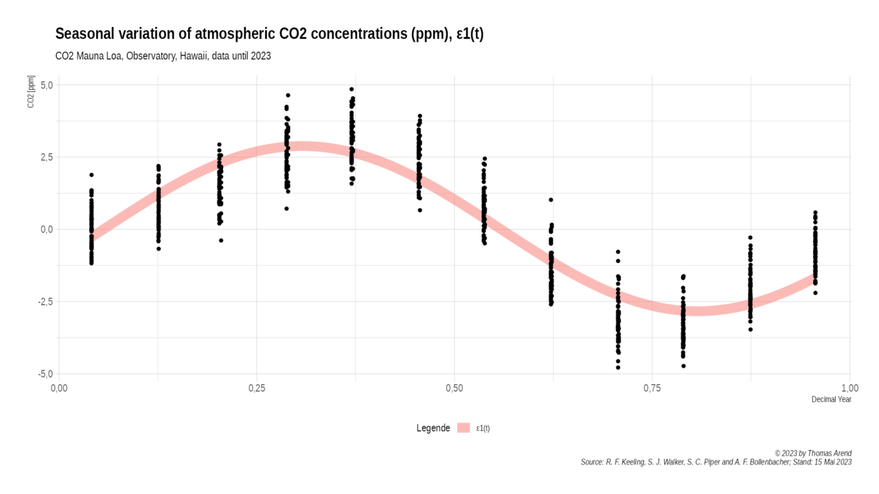
Diagram 2: Error ε₁(t) after Exponential Approximation
The visual inspection of the error function ε₁(t) shows a clear annual sinusoidal oscillation. Therefore adding the first sinusoidal part to our model should improve the accuracy of the approximation.

Error ε₂(t)

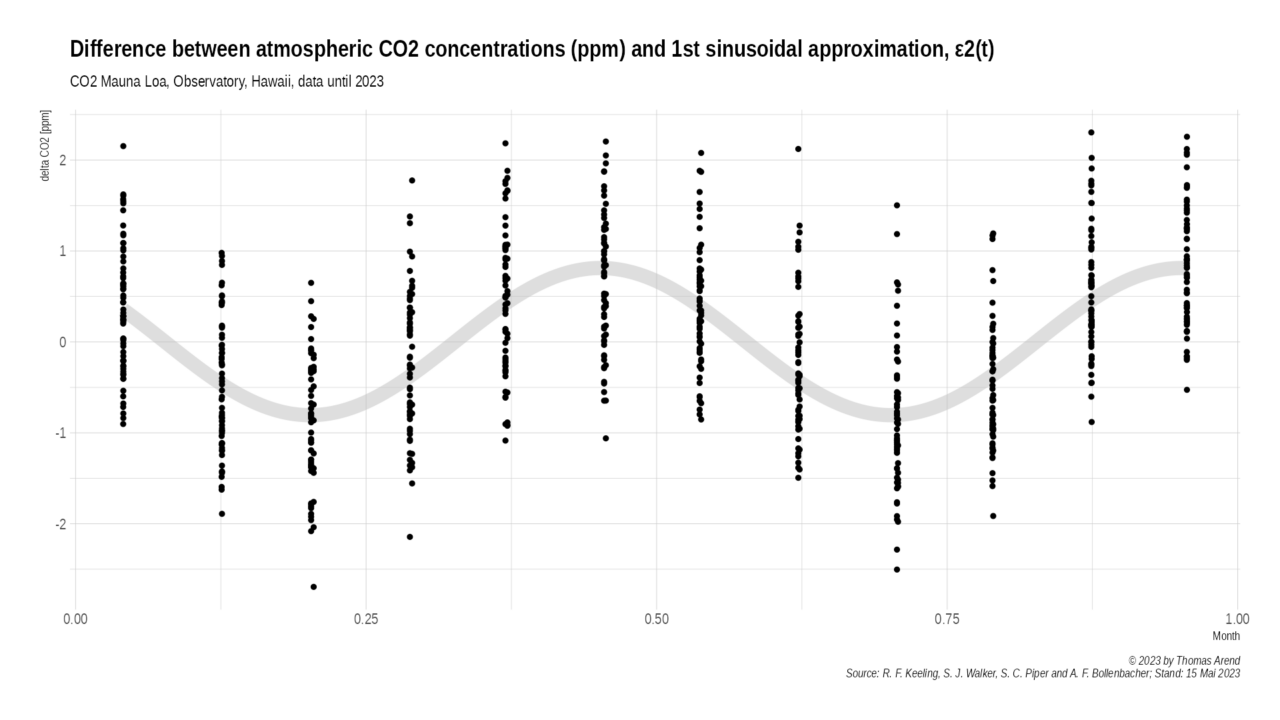
Diagram 3: Error ε₂(t) after Exponential and 1^st Sinusoidal Approximation

Our visual inspection of the error function ε₂(t) finds a semi-annual oscillation. This semi-annual oscillation explains the small deviations form the sinus function in the first error function.

Therefore we add a second sinusoidal part to our model to improve the approximation further.

Error ε₃(t)

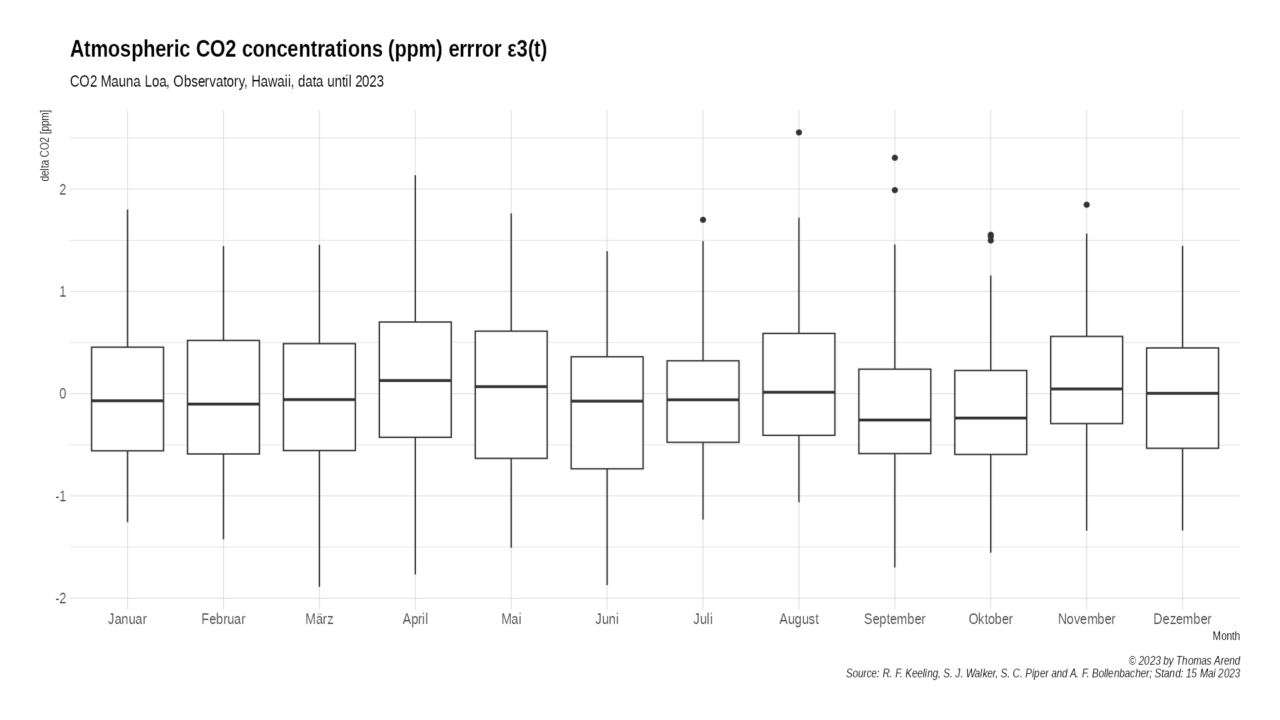
Diagram 4: Error ε₃(t) after Exponential, 1^st and 2^nd Sinusoidal Approximation

Our visual inspection of the error function ε₃(t) shows no obvious pattern. Therefore we stop at this point and do not add further parts to our model.

Extrapolation

To test the quality of the general model we restrict the data and extrapolate the approximation into the future. We determine the parameter of our model only on the values until December 1999 and call it Model 1999.

When we restrict the time frame from 1958 to 1999 the approximation differs only marginal.

CO2 (1999)(t) = 1.26738983189575e-12 * exp( 0.0160596707252981 * t )
+ 2.80725394368403 * sin( 2 * pi * ( t - 0.0617 ) )
- 0.750902310503362 * sin( 2 * pi * ( t - 0.0794 ) )
+ 256.03745907830

When we extrapolate this model we can »predict« the future CO₂ concentration and test the predictive power of this approach. For April 2023 we predict the CO₂ concentration to be 419.9 ppm. The real value was 422.73 ppm which is 2.83 ppm higher. Taking into account that approximation based on only 41 year and the prediction was more then 23 years in the »future« this is a very good guess.

Using both models to predict the values for December 2049 we calculate 506.5894 ppm with Model 1999 and 507.5627 ppm with Model 2023. These values are less than 1 ppm apart.

Diagram 5: Keiling Curve with Approximations based on values until December 1999

Diagram 5 visually shows that the extrapolation of the model fits extremely good with the real values.

Discussion

The proposed model provides a reasonable approximation of the monthly data of the Keeling Curve by combining an exponential function for the long-term trend and two sinusoidal functions for the annual and semi-annual oscillations. While the factors causing the annual oscillation can be attributed to natural processes such as plant growth and decay, the factors contributing to the second sinusoidal oscillation with the semi-annual frequency are not fully understood. Further research is needed to investigate the underlying mechanisms responsible for this phenomenon.

Limitations and Future Research

Although the proposed model captures the general behavior of the Keeling Curve, it is important to note that it may not account for all factors influencing CO₂ concentrations. The inclusion of additional sinusoidal components allows for a more accurate representation of the seasonal variations, but the underlying drivers of the semi-annual oscillations remain a subject of ongoing scientific inquiry. Future research efforts should focus on unraveling the complex interactions between various climatic, biological, and atmospheric processes that contribute to the observed semi-annual variations in CO₂ concentrations.

Conclusion

This study presents a mathematical model that combines an exponential function and sinusoidal functions to approximate the monthly data of the Keeling Curve. The model captures both the long-term trend and the annual variations in atmospheric CO₂ concentration, providing valuable insights into the impact of human activities and natural processes. However, the factors contributing to the second sinusoidal variation with the semi-annual oscillation require further investigation to enhance our understanding of the dynamics of CO₂ concentrations in the atmosphere.

When the approximation is extrapolated over a longer period using only data up to 1999, the predictive accuracy of the approach is impressive.

Limitations and Future Research

Although the proposed model captures the general behavior of the Keeling Curve, it is important to note that it may not account for all factors influencing CO2 concentrations. The inclusion of additional sinusoidal components allows for a more accurate representation of the seasonal variations, but the underlying drivers of the semiannual oscillations remain a subject of ongoing scientific inquiry. Future research efforts should focus on unraveling the complex interactions between various climatic, biological, and atmospheric processes that contribute to the observed semiannual variations in CO2 concentrations.

Conclusion

This study presents a mathematical model that combines an exponential function and a sinusoidal function to approximate the monthly data of the Keeling Curve. The model captures both the long-term trend and the seasonal variations in atmospheric CO2 concentration. The proposed approximation facilitates the analysis of CO2 concentration patterns and provides a valuable tool for understanding the dynamics of climate change and its underlying drivers.

Keywords

Keeling Curve, CO₂ concentration, exponential function, sinusoidal function, approximation, trend, seasonal variations, climate change.